Model Fitting

“All models are wrong but some are useful.” George Box

“Everything should be as simple as it can be, but not simpler.” Albert Einstein

Model is perhaps the most used term in a statistical context. A statistical model is means to capture the structure of the data as simply as possible. Put another way, our goal is to find the model that most efficiently and accurately summarizes how the data were generated.

Models are described via parameters and mathematical operators. Parameters are unobservable, but we can still estimate them and their effects by using the data we have. Estimation is how we determine the value of the parameters.

Frequentist estimation is the most common type. It assumes a parametric distribution and is interested in the long run of frequencies within the data. Most statistical software uses frequentist estimation—typically least squares estimation which involves minimizing the sum of squared errors. A more complex version is maximum likelihood estimation, or MLE which maximizes the log function by minimizing the negative log likelihood.

Monte Carlo estimation, or sometimes bootstrapping or resampling, requires very few assumptions and uses the observed data over and over to draw inferences.

Bayesian estimation assumes a parametric distribution. It also includes a prior distribution or prior knowledge about the parameter.

 

Linear Models

We use regression to predict a dependent variable from one or more independent variables. Regression gives us an equation that describes the form of the relationship between dependent and independent variables and predicts the value of the dependent variable based on the independent variable(s)

Ordinary Least Squares (OLS) regression

Ordinary least squares fits models of the form:

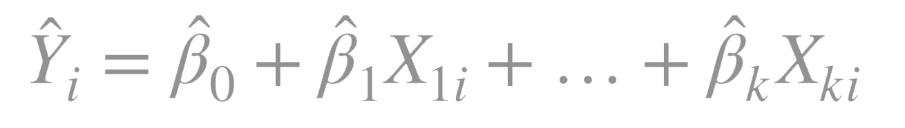
where \(n\) is the number of observations and \(k\) is the number of predictor variables.

\(\hat{Y}_i\) is the predicted value of the dependent variable for observation \(i\)

\(X_{ki}\) is the value of the \(k\)th independent variable for \(X = i\).

\(\hat{\beta}_0\) is the predicted value of \(Y\) when all the predictor variables are \(0\), i.e. the intercept.

\(\hat{\beta}_k\) is the slope representing the change in \(Y\) for a unit change in \(X_k\), i.e .the regression coeffient for the \(k\)th predictor.

When there is more than one predictor, we are dealing with multiple linear regression. When there is more than one independent variable, the regression coefficients indicate the increase in the dependent variable for a unit change in the independent variable, holding the other independent variables constant.

You can use the lm() function in R to fit an OLS regression model, and the summary() function to obtain model parameters and summary statistics.

Statistical assumptions underlying OLS regression

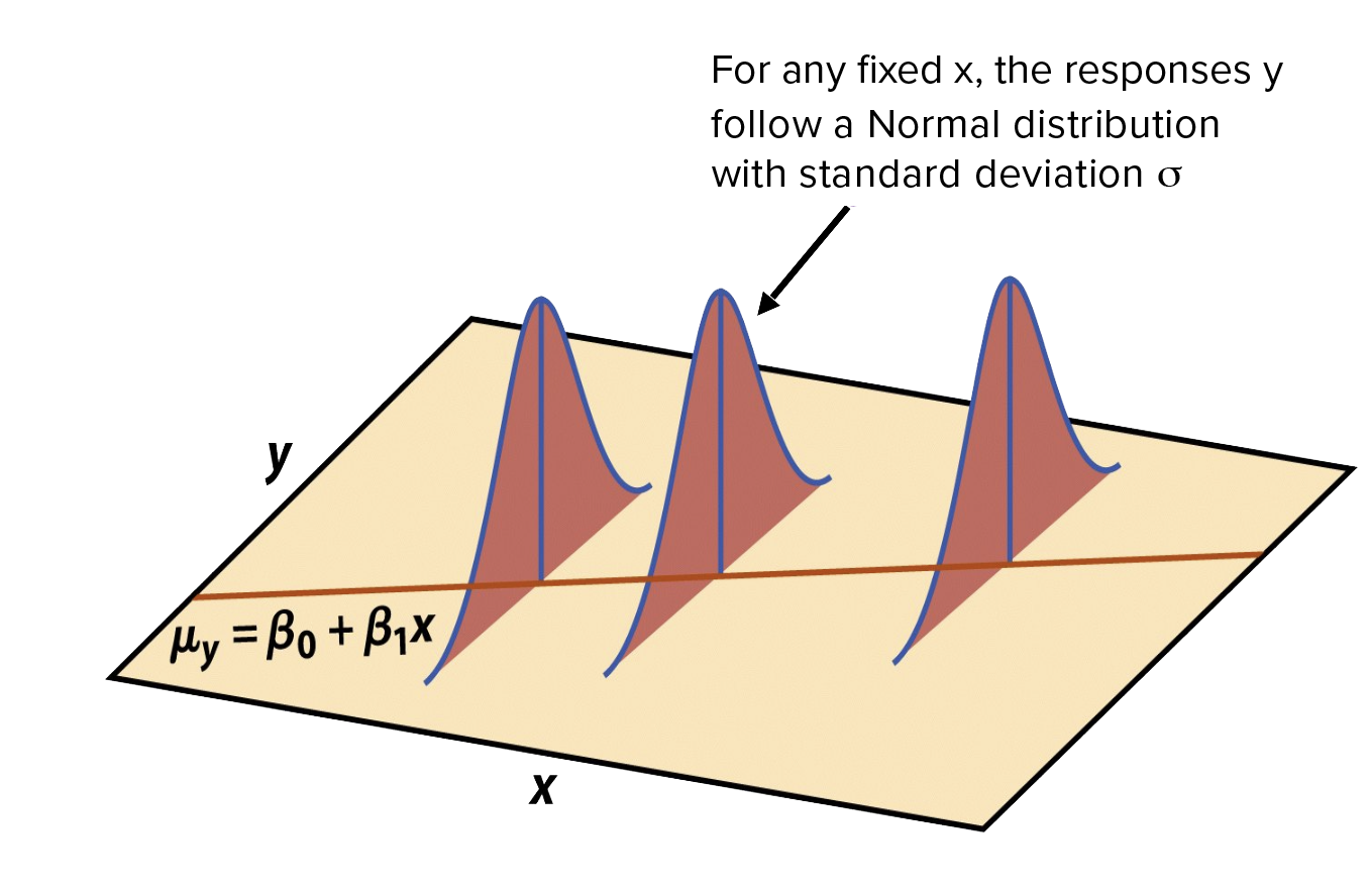
• Normality: For fixed values of \(X_{1 \dots n}\), \(Y\) is normally distributed

• Independence: The values of Y for a given X are independent of each other

• Linearity: The relationship between the independent variables and the dependent variable is linear

• Homoscedasticity: The variance of dependent variable is constant across all levels of the independent variable.

Regression Diagnostics

Applying the plot() functions to the model returned by lm() produces 4 graphs: (1) Residuals vs Fitted Values (2) Standardized residuals vs theoretical quantiles (Normal Q-Q plot) (3) Standardized residuals vs fitted values (4) Standardized residuals vs leverage.

• Normality: If the dependent variable is normally distributed for a fixed set of independent variable vales, the residuals should be normally distributed with a mean of 0. In this case, the points on the Q-Q plot should fall on a straight 45-degree line. You can also use the qqPlot() function in the car package to plot the studentized or jackknifed residuals against a \(t\) distribution with \(n - p - 1\) degrees of freedom where \(n\) is the sample size and \(p\) is the number of regression parameters including the intercept.

• Linearity: If the dependent variables is linearly related to the independent variables, there should be no systematic relationship between the residuals and the predicted values in plot 3.

• Homoscedasticity: If the homoscedasticity assumption is met, the points should form a random horizontal band around a horizontal line of best fit in plot 3. Heteroscedasticity is a systematic change in the spread of the residuals over the range of measured values. Heteroscedasticity is a problem because ordinary least squares (OLS) regression assumes that all residuals are drawn from a population that has a constant variance. Heteroscedasticity tends to be present in variables with a large range.

Dealing with violations of assumption

• Deleting outliers can often improve a dataset’s fit to the normality assumption. The largest outlier or influential observation is deleted, and the model is refit. If there are still outliers or influential observations, the process is repeated until an acceptable fit is obtained. Caution should be used when considering the deletion of observations.

• When models don’t meet the normality, linearity, or homoscedasticity assumptions, transforming one or more variables can often improve or correct the situation. Transformations typically involve replacing a variable \(Y\) with \(Y^{\lambda}\).

You can transform your data to address homoscedasticity

ANOVA

When factors are included as explanatory variables, the methodology is referred to as analysis of variance (ANOVA). An ANOVA that controls for the effects of at least one continuous covariate is referred to as analysis of covariance (ANCOVA). When there’s more than one dependent variable, the design is called a multivariate analysis of variance (MANOVA). If there are covariates present, it’s called a multivariate analysis of covariance (MANCOVA).

ANOVA and regression are both special cases of the general linear model. As with regression, the basic function for fitting a linear model is lm(). You can also use the aov() function. The results of lm() and aov() are equivalent.

The order in which the effects appear in a formula matters when there is more than one factor and the design is unbalanced, or covariates are present. By default, R employs the Type I (sequential) approach to calculating ANOVA effects. The greater the imbalance in sample sizes, the greater the impact that the order of the terms will have on the results. Given this, more fundamental effects should be listed earlier in the formula. The Anova() function in the car package provides the option of using the Type II or Type III approach, rather than the Type I approach used by the aov() function.

A significant anova F-test doesn’t tell you which treatments differ from one another. To answer this question you can use the TukeyHSD() function to test all pairwise differences between group means. You can plot the output of this function (all the pairwise comparisons) with the plot() function plot(TukeyHSD(aovmodel)). In addition, the effects package provides a powerful method of obtaining adjusted means for complex research designs and pre- senting them visually.

In a 2-way ANOVA with the presence of interactions, you can use the interaction.plot() function to display them.

Repeated Measures ANOVA

In repeated measures ANOVA, subjects are measured more than once. Running a repeated measures analysis of variance in R can be a bit more difficult than running a standard between-subjects anova. In repeated measures ANOVA, instead of using the same error term as the denominator for every entry in the ANOVA table, the repeated measures ANOVA uses different error terms as denominators and thus factor out subject differences. In R these error terms are the row labeled Residuals.

See this tutorial for more information on conducting repeated measures ANOVA in R.

You can conduct a repeated measures using the aov() function, and including an error term that contains the ‘subjects’ term, plus the within-subjects variables.

fitted_model <- aov(DV ~ IV + Error(Subject/IV), data=df)

Note that within-subject variables are entered twice in the main part of the model as well as in the ‘Error’ term, but between-subject variables are only entered once, in the main part of the model.

One drawback of this method is that it does not give any correction factors for violations of sphericity. It assumes that the variances of the differences between any two levels of the within-groups factor are equal. The degree to which sphericity is present, or not, is represented by a statistic called epsilon \(\epsilon\)). In real-world data, it’s unlikely that the sphericity assumption will be met. To address this you can use the Greenhouse-Geisser (GG) correction which estimates epsilon \(\hat{\epsilon}\) in order to correct the degrees of freedom of the \(F\)-distribution.

Another option is to use linear mixed effect models. Given that ANOVA is a linear model where the predictors are factors, we can run an ANOVA on a linear mixed model as follows using the lme4 package.

fitted_model <- lmer(DV ~ IV + (1|Subject), data=df).

Linear Mixed Effects Models

Introduction to linear mixed models

For random factors, you have three basic variants:

• Intercepts only by random factor: (1 | random.factor)

• Slopes only by random factor: (0 + fixed.factor | random.factor)

• Intercepts and slopes by random factor: (1 + fixed.factor | random.factor)

How to do Repeated Measures ANOVAs in R by Dominique Makowski

Mixed Models with R

R for Statistical Learning by David Dalpiaz. Chapter 4 Modeling Basics in R

Statistical Thinking for the 21st Century by Russell A. Poldrack. Chapter 5 Fitting models to data.

Data Science with R by Garrett Grolemund. Chapter 3 Model Fitting.

Model Selection

Model selection always involves a compromise between simplicity and predictive accuracy. All things being equal, given two models with approximately equal predictive accuracy, choose the simpler one.

You can compare the fit of two nested models using the anova() function. A nested model is one whose terms are completely included in the other model.

The Akaike Information Criterion (AIC) provides another method for comparing models. The index takes into account a model’s statistical fit and the number of parameters needed to achieve this fit. Models with smaller AIC values are preferred.